Project: Build Image Search

Intro

By the end of Part 2 of the Linear Algebra 101 for AI/ML series, we learned how to calculate the dot product, the definition of an embedding, and the application of embeddings to similarity search. In this article, Part 3 of the series, we're going to build an image search engine. Read this article, and complete the coding exercises in the free accompanying Google Colab notebook. Then run it for free on servers hosted by Google!

• Overview
• What is Google Colab?
• Brief Intro to Neural Networks
• CLIP – Contrastive Language-Image Pretraining
• Imagenette – mini-ImageNet
• Vector Database
• Similarity Search
• Cosine Similarity
• Conclusion

Overview

Building an image search engine consists of five main parts.

• First, we will download a pretrained neural network called CLIP.
• Then we will download a dataset of over 9000 images called Imagenette.
• Using the CLIP neural network, we will convert each of the 9000+ images into embeddings.
• We'll then store the embeddings in a special type of database called a vector database.
• Finally, we'll allow the user to input a query image so that we can search for and return similar images.

What is Google Colab?

Google Colab notebooks are executable documents that not only display text in Markdown but also run Python and command line code ¹. The beauty of using Colab is the notebooks run in Python environments preinstalled with widely used machine learning/data analysis Python modules (e.g., PyTorch, NumPy, etc.). This means you don't have to spend too much time setting up your dev environment, and instead, you can focus on building ML models and apps. Executable notebooks are also widely used in industry and academia, so notebook development is a useful skill to have on the resume. Best of all, it's free to use so that anyone with an internet connection and a Google account can access Google's computing resources for free. However, there are some restrictions, which you can learn more about in this Colab FAQ, but thankfully, those restrictions won't apply to the work we're tackling in this notebook ².

Brief Intro to Neural Networks

Let's briefly cover neural networks since we'll be using them to build our image search engine. We won't go into all the details in this article, so don't worry if you don't understand all of it. We'll build up intuition around neural networks in a future post.

Neural networks were once seen as a poor imitation of the human brain, but in 2012, researchers from the University of Toronto constructed a neural network architecture that was capable of producing significantly better results than all other non-neural network solutions for the ImageNet Challenge. That was the start of the deep learning revolution that grew and evolved into the generative AI technology wave of the early 2020s.

Neural networks consist of neurons and the connections between them, and they come in various arrangements, aka architectures. Below are three architectures you might have heard of: (vanilla) neural networks, convolutional neural networks (CNN), and GPT-1 (the precursor to GPT-4 and ChatGPT).

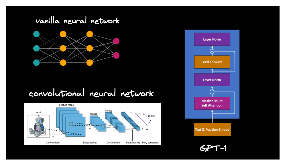
Not all pairs of neurons have a connection between them, but for those that do, the weight specifies the strength of the connection.

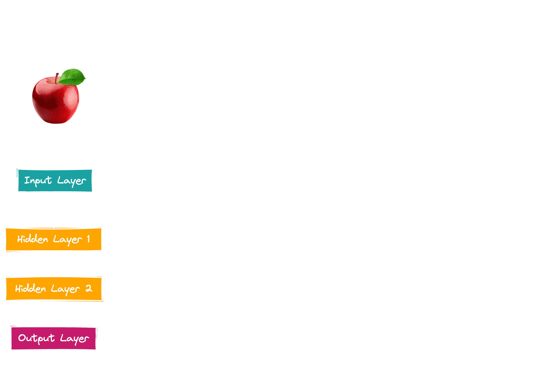
In the interactive diagram above, connections in light gray have a positive weight, and connections in fuchsia have a negative weight. When a neural network architecture is first initialized in a computer program, its neurons are arranged as specified by the architecture design, but its weights are often randomly initialized or drawn from a normal distribution. In this initial state, the neural network is unable to produce any useful output, so it must undergo a process called training. Upon completion of training, the weights are established such that the neural network is capable of producing useful output. It must be noted that there isn't just one set of weights such the neural network is considered trained. In fact, there are infinitely many sets of weights, so you just need to arrive at one set after training and that'll do.

So what actually happens during training? The neural network takes in an input, performs a bunch of mathematical calculations on that input, and produces an output. Then the training process compares the neural network's output to the expected output, aka the ground truth. Calculation of the difference between the ground truth and the output, aka the error, is then used to inform the neural network to adjust its weights such that the next time it sees this input, it'll generate an output closer to the ground truth.

To put it a different way, during training, the weights are adjusted little by little based on their relationship to the error, and eventually, training coerces the entire network of neurons and connections to be capable of producing useful output. The intricacies of how the error leads to adjustments to the weights is called backpropagation and will be covered in a future post on neural networks, but for now, it's enough to know that training a neural network is somewhat similar to training a student with many quiz questions and marking the wrong answers such that the student will hopefully answer the questions correctly the next time around. If you're still curious how backpropagation works, this YouTube video by Artem Kirsanov is a fantastic visual explanation.

CLIP – Contrastive Language-Image Pretraining

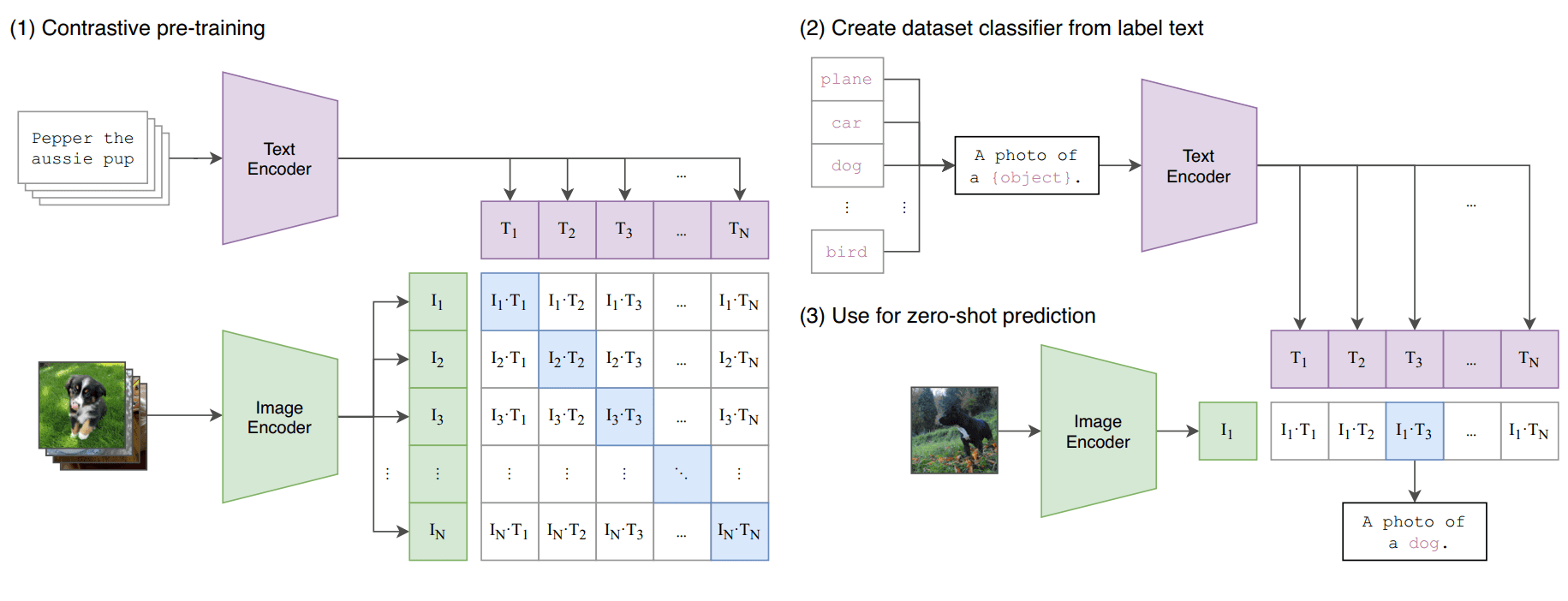
CLIP, which stands for Contrastive Language-Image Pretraining, is a specific neural network architecture that was released by OpenAI in 2021. This architecture allows the neural network to process both text (aka language) and images (aka vision). Because it can process two different modalities, we call it a language and vision multimodal model. Below is a diagram from OpenAI showing how CLIP was trained.

As mentioned above, knowing the neural network architecture alone is not enough for the model to be useful. We must possess a set of weights. Unfortunately for hobbyists, practitioners, and institutions with few resources, training a neural network from scratch to obtain a set of good, useful weights can be prohibitively expensive these days for extremely large neural networks. The number of neurons and connections in state of the art models have increased exponentially in recent years such that the largest models contain 100s of billions or trillions of weights. The computing power needed to adjust all these weights while training on billions of data points can cost 100s of millions or billions of US dollars. Fortunately, some AI research labs have taken on the cost of training such models and have released the weights to the public. Neural networks that come preloaded with useful weights are called pretrained models.

For starters, we're going to download a set of weights for the CLIP model.

model = CLIPModel.from_pretrained("openai/clip-vit-base-patch32")

As a recap, CLIP is a language and vision multimodal model, which means it accepts both text and image inputs. However, before you can give it any text or image input, you must use a processor to prepare the input for the model.

processor = CLIPProcessor.from_pretrained("openai/clip-vit-base-patch32")

CLIPProcessor is actually a wrapper class around an image processor and a text processor.

• If CLIP is given text input, a tokenizer converts the input text to a vector that can be understood by the model.
• If CLIP is given image input, an image processor resizes, crops, and tweaks the image pixel values so that they're suitable for the model.

You can learn more about the processor here.

Let's play around with the CLIP model to understand what it's capable of doing.

import requests
url = "http://images.cocodataset.org/val2017/000000039769.jpg"
image = Image.open(requests.get(url, stream=True).raw)
inputs = processor(images=image, return_tensors="pt")
image_features = model.get_image_features(**inputs)

In the code above, we follow an example from the Hugging Face documentation by downloading an image containing two cats. Then we process the image by feeding it into CLIP, and storing the output embedding in image_features. Complete the coding activities below before continuing.

Above, we fed CLIP a 224x224 pixel image as input, and its output was a 512-dimensional embedding. The embedding is useless on its own, but when compared to other 512-dimensional embeddings output by the same CLIP model loaded with the same set of weights, the embedding begins to take on meaning.

Imagenette – mini-ImageNet

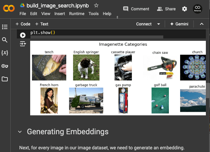
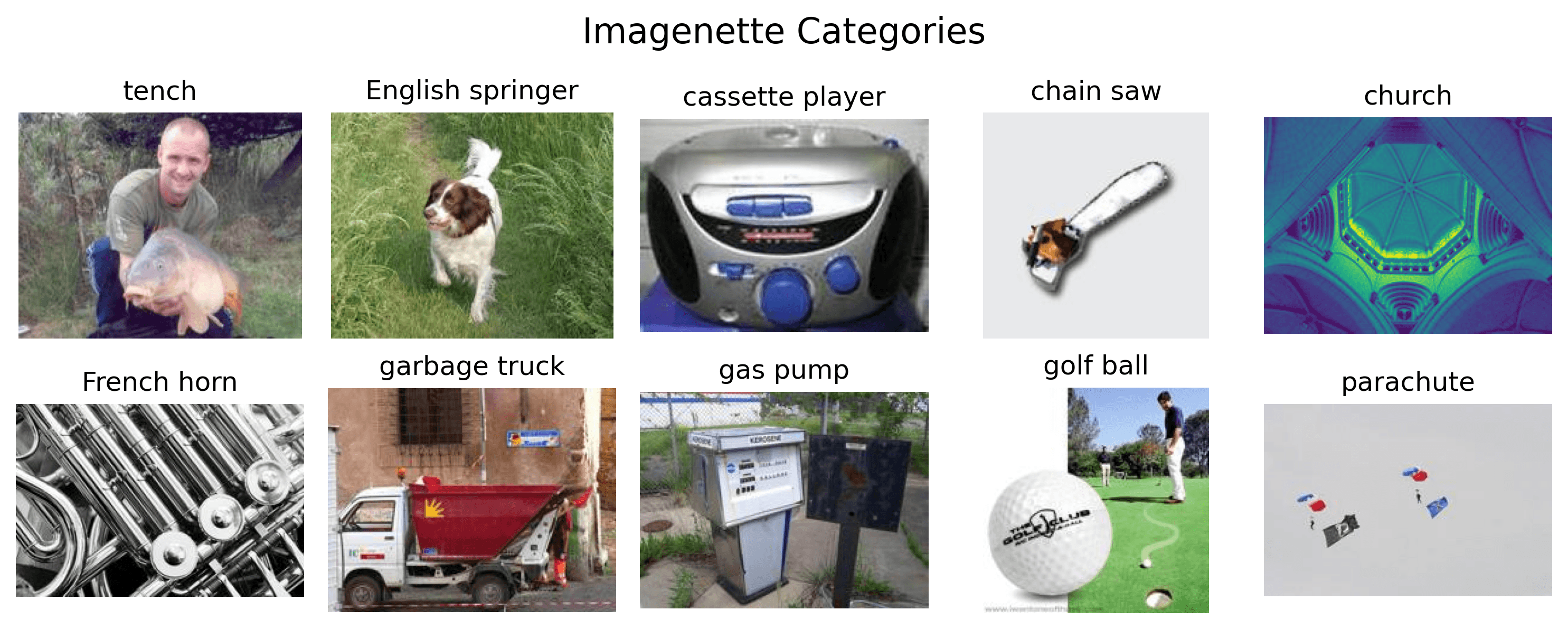
ImageNet is a visual database of over 14 million images containing more than 20,000 categories of objects such as sunglasses, bassinet, and mongoose. While we could try to build an image search engine across these 14 million images, for pedagogical purposes, we're going to use a subset of ImageNet called Imagenette, which is a dataset that contains just 10 categories from ImageNet's 20,000. Click here to download the 160 pixel variant of the dataset, which is about 88.3MB in size (the Google Colab notebook contains download instructions as well).

Once you finish downloading it, open up the zip file and take a look at the dataset structure:

$ tree -L 2 imagenette2-160
imagenette2-160
├── noisy_imagenette.csv
├── train
│   ├── n01440764
│   ├── n02102040
│   ├── n02979186
│   ├── n03000684
│   ├── n03028079
│   ├── n03394916
│   ├── n03417042
│   ├── n03425413
│   ├── n03445777
│   └── n03888257
└── val
    ├── n01440764
    ├── n02102040
    ├── n02979186
    ├── n03000684
    ├── n03028079
    ├── n03394916
    ├── n03417042
    ├── n03425413
    ├── n03445777
    └── n03888257

23 directories, 1 file

You see the dataset consists of train and val directories, which stand for training and validation datasets, but we'll focus on just the images located within train. Inside train, there are 10 subdirectories, each of which contains a category of images (see categories above).

In Coding Exercise 1 of the Google Colab notebook, you will generate a CLIP embedding for each of the images in the train dataset.

Vector Database

Now that we have the embeddings of the images, we need to store them in a vector database. There are many benefits to storing embeddings in a vector database over a standard relational database:

• Efficient similarity search: Vector databases are optimized for high-dimensional vector data and can perform fast similarity searches. This is crucial for image retrieval based on visual similarity.
• Scalability: Vector databases are designed to handle large volumes of high-dimensional data, making them more suitable for storing and querying millions or billions of image embeddings.
• Specialized indexing: Vector databases use specialized indexing structures that are tailored for vector data, enabling faster retrieval compared to traditional indexing methods used in relational databases.
• Native support for vector operations: Vector databases provide built-in functions for vector operations like cosine similarity, Euclidean distance, and dot product, which are essential for comparing image embeddings.

The rise of AI/ML and embeddings has led to an increase in vector database services. Pinecone is one of the most well known ones, and we focus on it in this article because of their free tier.

First, create a Pinecone index, which you will complete in Coding Exercise 2.

Now that you have an index, you can upload vectors to it. Simply call the upsert method.

index.upsert(
  vectors=[
    {"id": "/path/to/img1", "values": [-0.12, 0.05, -0.23, 0.18, -0.07, 0.31]},
    {"id": "/path/to/img2", "values": [0.42, -0.19, 0.27, -0.35, 0.11, -0.28]},
    {"id": "/path/to/img3", "values": [-0.51, 0.63, -0.17, 0.45, -0.38, 0.22]},
    {"id": "/path/to/img4", "values": [0.78, -0.41, 0.56, -0.72, 0.89, -0.25]}
  ]
)

In the example above, CLIP embeddings have already been generated for each image so that they can be uploaded to a vector database. You'll complete this task in Coding Exercise 3.

Similarity Search

Now that we have image embeddings uploaded to a vector database, all that's left is to compare user query images with those stored in our database and to find and return the most similar images. Pause and think for a moment how you'd do that. Go ahead and tackle Coding Exercise 4 if you have an idea. If not, read on!

Now that we have a vector database full of embeddings, it'd make sense to compare each of those embeddings of the query image's embedding by using the dot product. While using a brute force for-loop may accomplish the job, it won't scale as the vector database holds more and more embeddings (such as 1 billion embeddings). As you read above, modern vector databases use more efficient algorithms to run the dot product at scale across millions and billions of vectors. One of the biggest open source contributions came from Facebook in 2017, when they released Faiss, which stands for Facebook AI Similarity Search. This software enabled the first similarity search across 1 billion high dimensional vectors, which contributed to the rise of vector databases. Pinecone gives us this powerful functionality with an index query function:

query_vector = [0.23, -0.21, 0.36, -0.92, 0.19, -0.23]
index.query(
    namespace="my-namespace",
    vector=query_vector,
    top_k=3,
    include_values=True
)

In the function call above, assuming the vector database contains many embeddings of the same dimension, the query function will ask Pinecone to search for the three embeddings most similar to the query_vector (the top_k parameter specifies the number of embeddings to return). Underneath the hood, Pinecone is using Faiss or some variant of it as well as other optimizations so that the dot product can be used to compare the query_vector against many other embeddings in an efficient manner.

Cosine Similarity

The dot product between two embeddings is one measure we can use to measure similarity. But there are also other similarity metrics. Let's learn about cosine similarity. In Part 2, we learned about the cosine formula for the dot product.

Let's divide both sides of the equation by $|{\color{cyan}{\vec{a}}}||{\color{orange}{\vec{b}}}|$:

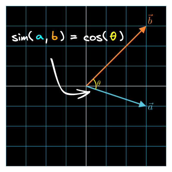
Now we have an equation that tells us the cosine similarity between two vectors. As its name suggests, this number is a measure of similarity – it determines whether two vectors are pointing in roughly the same direction. You can play with the Interactive Dot Product Playground below if you want to see how the $\cos({\color{yellow}{\theta}})$ varies as two vectors change directions.

The cosine similarity is often used as a measure of semantic similarity between two embeddings and when you don't want to include vector magnitude in similarity calcuations. If you need a refresher on these concepts, head over to Part 2 of the Linear Algebra 101 for AI/ML series.

Conclusion

That's it! Congratulations on learning how to build an image search engine. Together with Part 1 and Part 2 of the Linear Algebra 101 for AI/ML series and the Google Colab notebook that accompanies this article, you've learned the absolute basics of linear algebra and PyTorch and applying that new knowledge toward building a useful image search engine.