Linear Algebra 101 for AI/ML – Part 2

Intro

In Part 1 of this Linear Algebra 101 for AI/ML Series, we learned about the fundamental building blocks of linear algebra: vectors and matrices. We learned how element-wise operations apply to the vector/matrix's individual elements independently, and then we played around with these mathematical building blocks using an open source ML framework called PyTorch, widely used in academia and industry.

In this article, Part 2 of the series, we will build on that foundational knowledge. First, we will cover an operation that applies to the vector/matrix's individual elements as a whole: the dot product. This operation belongs to a class of operations that do not view the individual elements independently. Then we will visualize the dot product operation to build intuition, and finally, we will learn about embeddings, which are special types of vectors that represent concepts, objects, and ideas. Embeddings are used throughout modern AI and have applications in large language models, image generation models, and recommendation systems. In the article, you will find questions, a quiz, and two interactive playgrounds (the Interactive Dot Product Playground and the Interactive Embedding Explorer are best viewed on laptop/desktop) that were designed to help you understand the concepts.

In Part 3 of the series, we will use all the fundamental linear algebra we will have learned in Part 1 and Part 2 to build an image search engine. Below is a preview of the image search engine, which returns images similar to the user's input image.

Without further ado, let's get started!

Dot Product

We will approach the dot product from two perspectives: an algorithmic perspective and a visual one.

Algorithmic Perspective

Below are two vectors, ${\color{cyan}{\vec{a}}} \in \mathbb{R}^{\color{fuchsia}{4}}$ and ${\color{orange}{\vec{b}}} \in \mathbb{R}^{\color{fuchsia}{4}}$ .

\left. {\color{cyan}{\vec{a}}} = \begin{bmatrix} 1 \\ 2 \\ 4 \\ 8 \\ \end{bmatrix} \quad {\color{orange}{\vec{b}}} = \begin{bmatrix} 1 \\ 0.5 \\ 0.25 \\ 0.125 \\ \end{bmatrix} \quad \right\}{\color{fuchsia}{4}} \text{ rows}

The notation for the dot product is simply a dot between two vectors: ${\color{cyan}{\vec{a}}} \cdot {\color{orange}{\vec{b}}}$ . The algorithm for calculating a dot product is simply to sum the products of corresponding pairs between two vectors. Let's break down what that means. First, let's calculate the products:

\begin{bmatrix} {\color{cyan}{1}} \\ {\color{orange}{2}} \\ {\color{yellow}{4}} \\ {\color{magenta}{8}} \\ \end{bmatrix} \cdot \begin{bmatrix} {\color{cyan}{1}} \\ {\color{orange}{0.5}} \\ {\color{yellow}{0.25}} \\ {\color{magenta}{0.125}} \\ \end{bmatrix} \Rightarrow \begin{array}{l} {\color{cyan}{1}} \cdot {\color{cyan}{1}} \\ {\color{orange}{2}} \cdot {\color{orange}{0.5}} \\ {\color{yellow}{4}} \cdot {\color{yellow}{0.25}} \\ {\color{magenta}{8}} \cdot {\color{magenta}{0.125}} \\ \end{array}

Next, we sum the products:

{\color{cyan}{1}} \cdot {\color{cyan}{1}} + {\color{orange}{2}} \cdot {\color{orange}{0.5}} + {\color{yellow}{4}} \cdot {\color{yellow}{0.25}} + {\color{magenta}{8}} \cdot {\color{magenta}{0.125}} = 4

Thus, ${\color{cyan}{\vec{a}}} \cdot {\color{orange}{\vec{b}}} = 4$ . Let's see how to calculate the dot product with PyTorch.

Python

>>> a = torch.tensor([1.0, 2.0, 4.0, 8.0])
>>> b = torch.tensor([1.0, 0.5, 0.25, 0.125])

>>> torch.dot(a, b)
tensor(4.)

To put it another way, to calculate the dot product, first we use the element-wise multiply operation, and then we sum up the products. Just for fun, let's implement torch.dot with native Python:

Python

>>> sum([a[i] * b[i] for i in range(len(a))]) # Python implementation of dot product
tensor(4.)

Concept Check

How would you implement torch.dot with PyTorch element-wise operations (Hint: Look at the documentation for torch.sum)?

Remember, the dot product is the sum of the product of its elements.

Python

>>> a = torch.tensor([1.0, 2.0, 4.0, 8.0])
>>> b = torch.tensor([1.0, 0.5, 0.25, 0.125])

# Solution
>>> temp = a*b # First, we element-wise multiply to get a list of products
>>> dot_product = temp.sum() # Then, we sum up the products
>>> dot_product == torch.dot(a, b) # Testing our implementation
>>> tensor(True)

# More concise solution
>>> (a*b).sum() == torch.dot(a, b) # 1 line of code
>>> tensor(True)

Visual Perspective

At this point, you're probably wondering: what does the dot product mean? Is there any meaning behind element-wise multiplying two vectors and then summing up the products? To aid our understanding of the dot product visually, let's introduce another way to calculate the dot product. This second equation for calculating the dot product is called the cosine formula for the dot product.

\vec{a} \cdot \vec{b} = |\vec{a}||\vec{b}|\cos(\theta)

(We won't cover why these two values are equivalent, but the proof can be found here.)

Vector Norm

There's some slightly new notation in the cosine formula for the dot product, so let's take a brief pause to understand it. In the cosine formula, $|\vec{a}||\vec{b}|\cos(\theta)$ , you'll notice vertical bars surrounding each vector. A vector paired with vertical bars, $|\vec{a}|$ , is called the norm of the vector. The norm of a vector measures its length or magnitude. To calculate the norm, let's rewrite what a general vector looks like:

\left. {\color{cyan}{\vec{a}}} = \begin{bmatrix} a_0 \\ a_1 \\ \vdots \\ a_{{\color{orange}{n}}-1} \\ \end{bmatrix} \in \mathbb{R}^{\color{orange}{n}} \right\}\text{{\color{orange}{n}} rows}

The norm of the vector is:

|{\color{cyan}{\vec{a}}}| = \sqrt{a_0^2 + a_1^2 + \cdots + a_{{\color{orange}{n}}-1}^2}

To understand why the equation above calculates the magnitude of the vector, let's visualize a vector, ${\color{yellow}{\vec{v}}}$ , in 2D space, a dimension much friendlier to human intuition than $N$ -dimensional space.

We see that ${\color{yellow}{\vec{v}}}$ has its tail at the origin $(0,0)$ and its head at $(2,3)$ . If physicists were viewing ${\color{yellow}{\vec{v}}}$ , then they would imagine it as a force that pushes an object from $(0,0)$ to $(2,3)$ . In other words, we'd say that the object's final position is 2 steps to the right along the ${\color{orange}{\vec{x}}}$ axis and 3 steps up along the ${\color{cyan}{\vec{y}}}$ axis. However, just because its final position is at $(2,3)$ does not mean it first traveled 2 steps to the right along the ${\color{orange}{\vec{x}}}$ axis, and then 3 steps up along the ${\color{cyan}{\vec{y}}}$ axis. Instead, it traveled along the straight yellow line from $(0,0)$ to $(2,3)$ . How do we calculate the distance of this straight line?

Notice that ${\color{yellow}{\vec{v}}}$ , ${\color{orange}{\vec{v_x}}}$ , and ${\color{cyan}{\vec{v_y}}}$ form a triangle, with ${\color{yellow}{\vec{v}}}$ as the hypotenuse. We use the Pythagorean theorem we learned in grade school, $a^2 + b^2 = c^2$ , to calculate the length of ${\color{yellow}{\vec{v}}}$ , aka the norm of ${\color{yellow}{\vec{v}}}$ .

\begin{align*} (\text{Length of } {\color{yellow}{\vec{v}}})^2 &= {\color{orange}{v_x}}^2 + {\color{cyan}{v_y}}^2 \\ \text{Length of } {\color{yellow}{\vec{v}}} &= \sqrt{{\color{orange}{v_x}}^2 + {\color{cyan}{v_y}}^2} \\ |{\color{yellow}{\vec{v}}}| &= \sqrt{{\color{orange}{v_x}}^2 + {\color{cyan}{v_y}}^2} \end{align*}

Now imagine if ${\color{yellow}{\vec{v}}}$ were a vector in 3D space. Its norm would be:

|{\color{yellow}{\vec{v}}}| = \sqrt{{\color{orange}{v_x}}^2 + {\color{cyan}{v_y}}^2 + {\color{magenta}{v_z}}^2}

Finally, generalizing to $N$ -dimensional space, we have the equation we saw earlier:

|{\vec{v}}| = \sqrt{{v_0}^2 + {v_1}^2 + \cdots + {v_{N-1}}^2}

Now that we are familiar with the notation, let's revisit the cosine formula for the dot product:

\vec{a} \cdot \vec{b} = |\vec{a}||\vec{b}|\cos(\theta)

The reason why we introduced this new cosine formula is it allows us to interpret the dot product geometrically.

Interactive Dot Product Playground

Before we dive into the explanation of the cosine formula for the dot product, let's first play around with an interactive playground that allows you to drag the arrowhead of the vectors around in a 2D number plane (only works on laptop/desktop!). Go ahead and try it out. See how the dot product between vector 1 and vector 2 changes (see the dynamic value of the dot product in the panel). Dragging the arrowheads around allows you to change the angle between the vectors and their lengths. As the cosine formula states, both angle and length (aka norm) have an impact on the dot product.

Vector 1:

(-3.00, 3.00)

Norm 1:

4.24

Vector 2:

(3.00, 2.00)

Norm 2:

3.61

Dot Product:

-3.00

cos(θ):

-0.1961

Tip: Click and drag the arrowheads to move the vectors on laptop/desktop

Have you played around with the interactive playground? If so, now it's time to understand the dot product.

Subscribe for more Linear Algebra 101 and access to a free Google Colab notebook that walks you through step by step how to build an ML image search engine. Unsubscribe any time.

Here, we see two vectors $\color{cyan}{\vec{a}}$ and $\color{orange}{\vec{b}}$ with an angle of $\color{yellow}{\theta}$ between them.

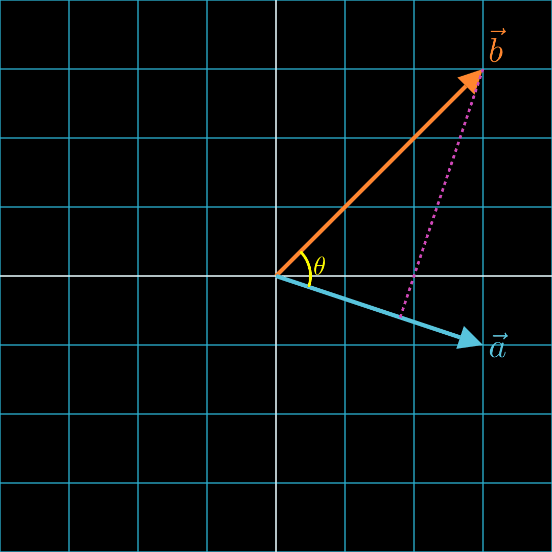
Let's draw a dotted line from the tip of $\color{orange}{\vec{b}}$ to $\color{cyan}{\vec{a}}$ such that the dotted line is at $90^\circ$ angle to $\color{cyan}{\vec{a}}$ .

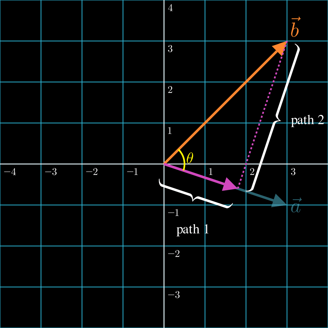
Imagine two forces. The first force moves an object from the origin, $(0,0)$ , along path 1. The second force then takes over and moves the object along path 2. The object would end up at $(3,3)$ . Notice that the force that pushes the object along path 1 is in the same direction as $\color{cyan}{\vec{a}}$ . In other words, it's aligned with $\color{cyan}{\vec{a}}$ . 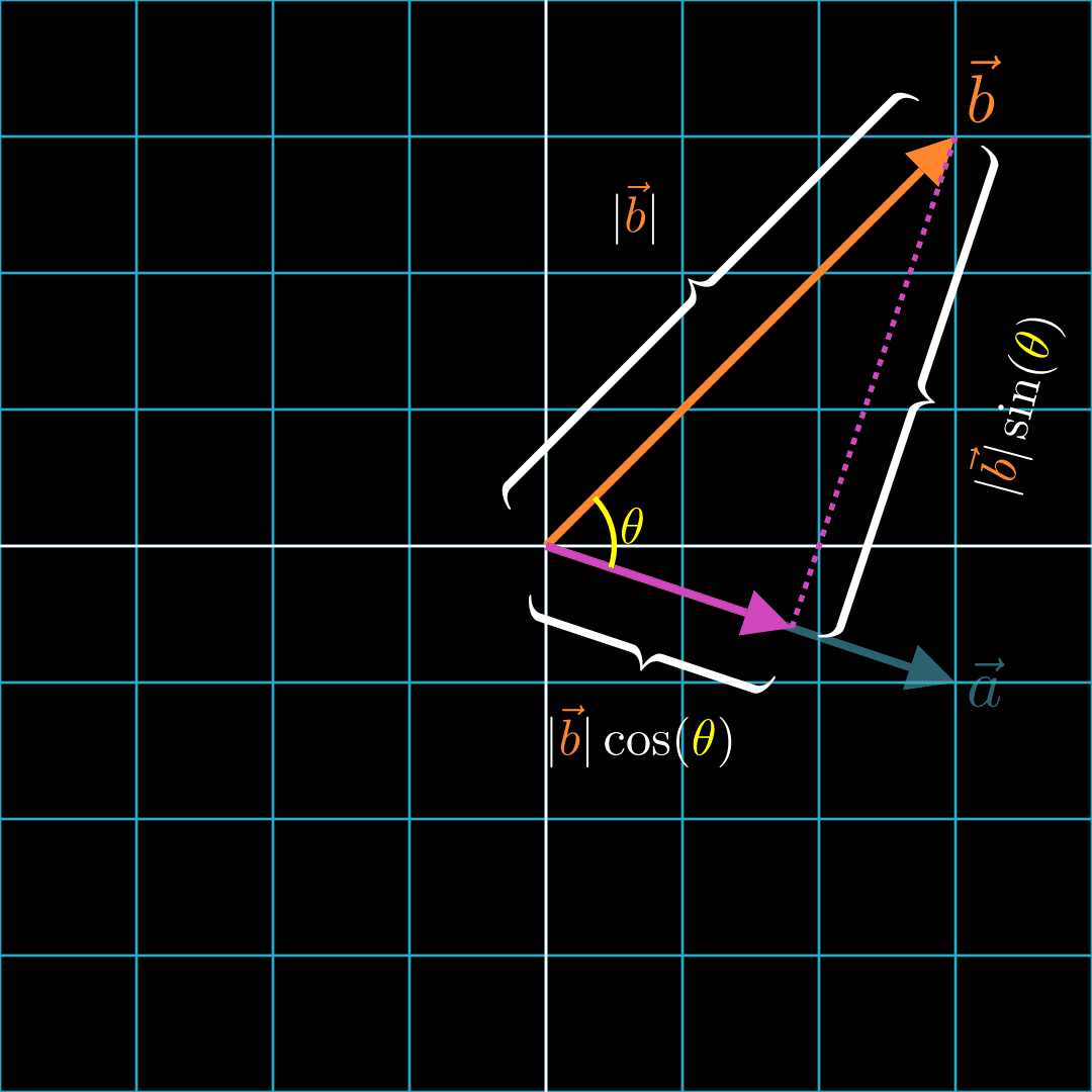This component is called the projection of $\color{orange}{\vec{b}}$ onto $\color{cyan}{\vec{a}}$ .

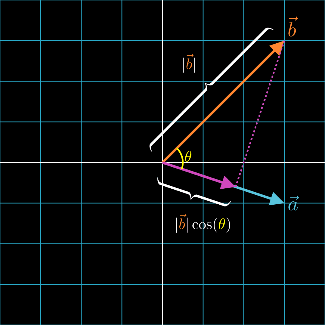
Since path 1, path 2, and $\color{orange}{\vec{b}}$ make a right triangle, we can calculate the lengths of the paths with trigonometry. We see that the projection of $\color{orange}{\vec{b}}$ onto $\color{cyan}{\vec{a}}$ has a length of $|{\color{orange}{\vec{b}}}| \cos({\color{yellow}{\theta}})$ .

{\color{cyan}{\vec{a}}} \cdot {\color{orange}{\vec{b}}} = |{\color{cyan}{\vec{a}}}| |{\color{orange}{\vec{b}}}| \cos({\color{yellow}{\theta}})

Now we see that multiplying $|{\color{cyan}{\vec{a}}}|$ and $|{\color{orange}{\vec{b}}}| \cos({\color{yellow}{\theta}})$ is essentially the same as multiplying the length of ${\color{cyan}{\vec{a}}}$ and the length of the component of ${\color{orange}{\vec{b}}}$ along the direction of ${\color{cyan}{\vec{a}}}$ . That means, the more ${\color{cyan}{\vec{a}}}$ and ${\color{orange}{\vec{b}}}$ are aligned and pointing in the same direction, the higher the dot product. The less they are aligned, the smaller the dot product. Let's take a look at some cases below.

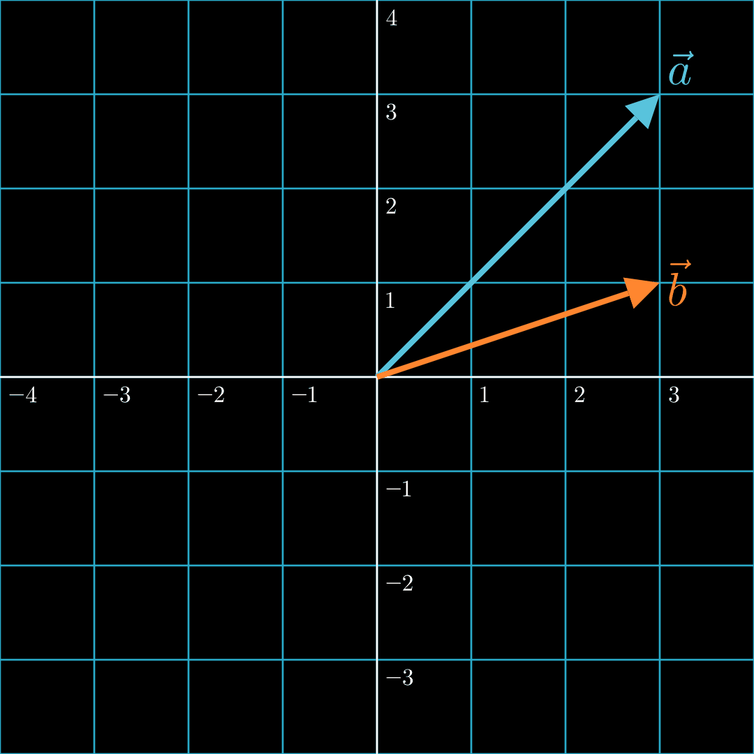
{\color{cyan}{\vec{a}}} \cdot {\color{orange}{\vec{b}}} > 0

In this case, the two vectors are generally aligned and pointing in the same general direction. Formally, the angle between the two vectors is less than 90°. Hence, a positive dot product.

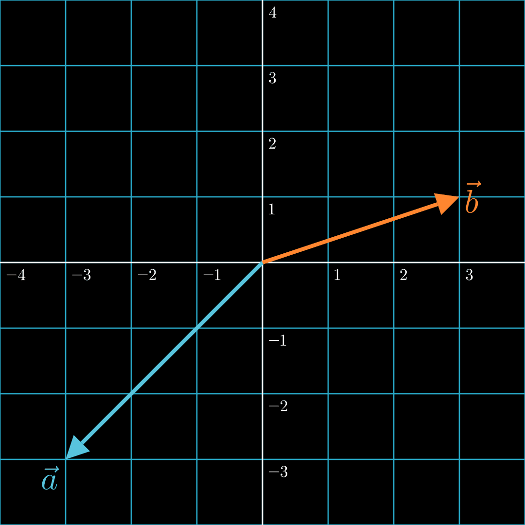
{\color{cyan}{\vec{a}}} \cdot {\color{orange}{\vec{b}}} < 0

In this case, the two vectors are generally not aligned and pointing in roughly opposite directions. Formally, the angle between the two vectors is greater than 90° and less than 270°. Hence, a negative dot product.

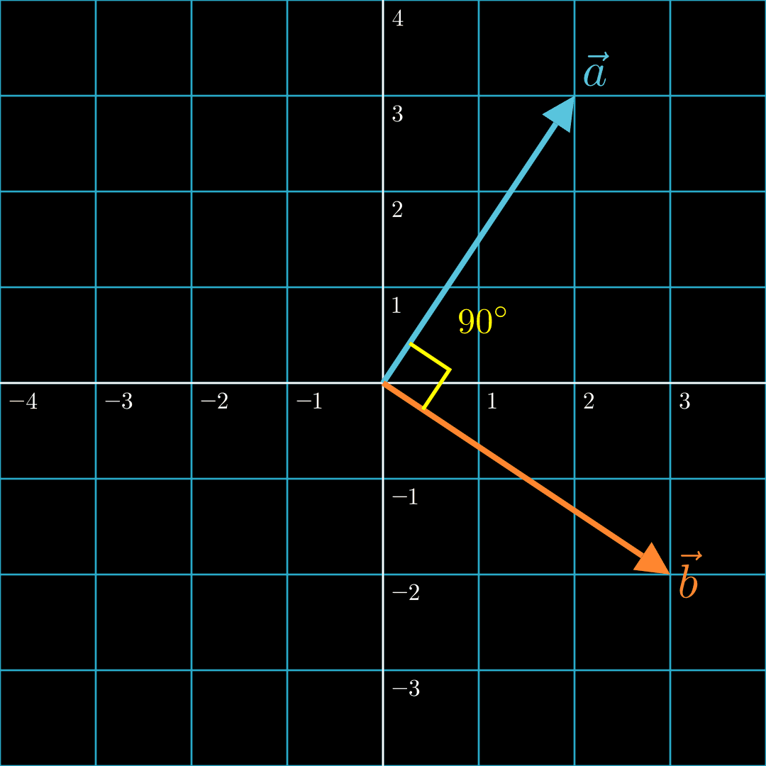
{\color{cyan}{\vec{a}}} \cdot {\color{orange}{\vec{b}}} = 0

In this case, the two vectors are perpendicular. They are neither aligned nor misaligned. Thus, the dot product is zero.

Don't worry if you're still trying to grasp these concepts. We just covered a lot of math. You can go back to the Interactive Dot Product Playground above to build intuition around the relationship between the dot product and the lengths and direction of vectors.

Embeddings

How does any of this math apply to machine learning? It turns out our new knowledge of vectors and dot products can be applied to large language models like ChatGPT, image generation like DALLE, and movie recommendation systems like Netflix.

As we will learn in a future article, AI applications based on neural networks do not process images, text, video, and audio directly. Instead, these inputs are first converted to vectors and matrices, and then these vectors and matrices are passed into the neural networks, which can perform various mathematical operations on them before producing output such as a chatbot response, a synthetically generated image, or a recommended movie. Even though to human eyes these vectors and matrices might seem like random but organized lists of numbers, to the neural network, they contain concepts. Vectors that represent these concepts are called embeddings. Because the seemingly random numbers in the vectors are capable of representing anything from a bird to electric cars to globalization, we say that these embeddings capture semantic meaning.

To illustrate, let's take a look at three popular movies. Suppose The Avengers: Endgame is represented by a vector that spans from the origin $(0, 0)$ to $(3, 3)$ , Spiderman by a vector that points to $(3, 1)$ , and La La Land by a vector that points to $(-3, -2)$ . Alternatively but subtly, we can view these movies as just the points at the end of the vector as opposed to the entire vector (e.g., Spiderman is just $(3, 1)$ as opposed to the vector pointing to $(3, 1)$ ). These are equivalent representations.

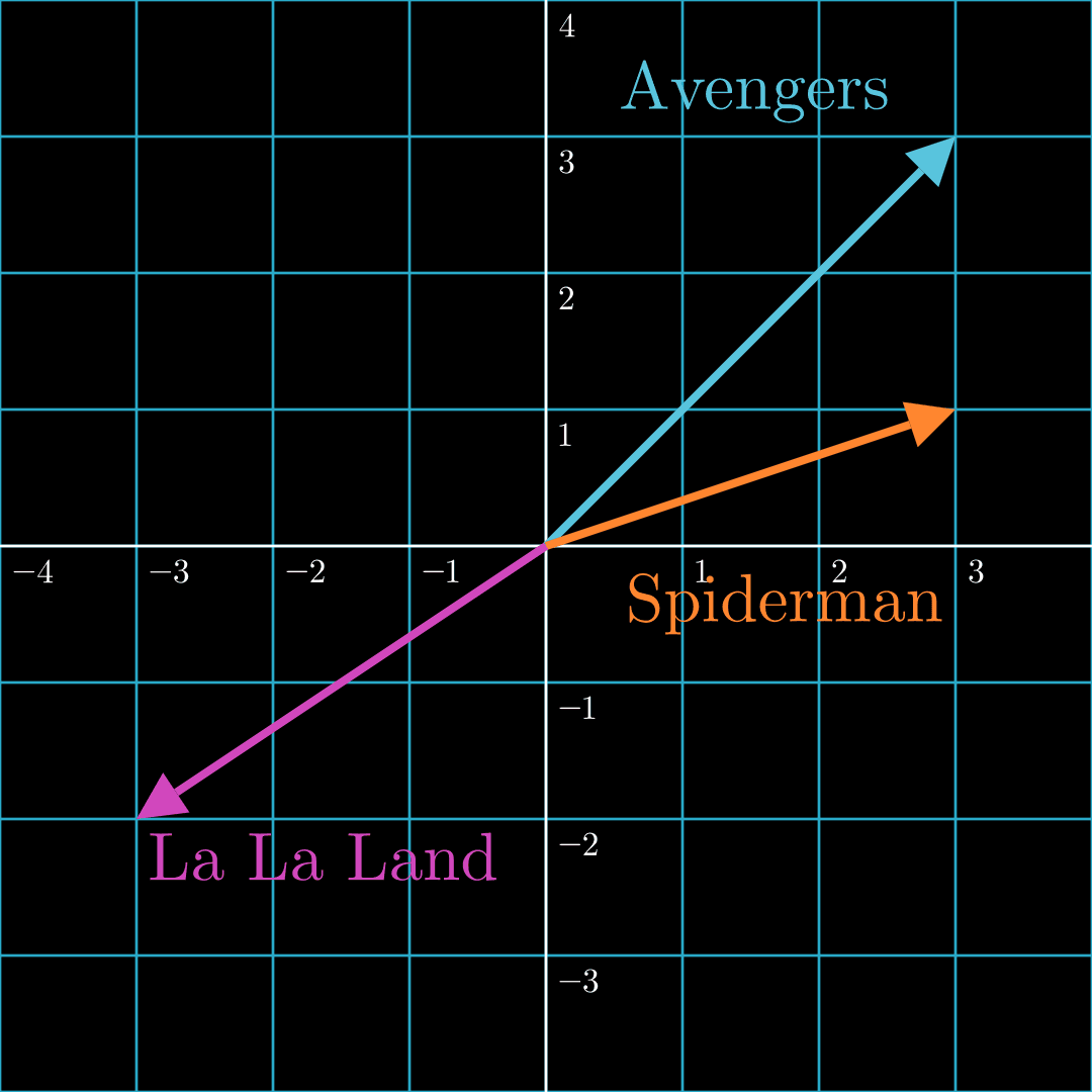
{\color{cyan}{\vec{A}}} \cdot {\color{orange}{\vec{S}}} > 0 \\ {\color{cyan}{\vec{A}}} \cdot {\color{magenta}{\vec{L}}} < 0 \\

Since The Avengers: Endgame and Spiderman are Marvel superhero movies, their vectors would be roughly aligned and thus their dot product would be positive. However, the movie La La Land has less action and a more serious overtone. Thus its dot product with the other two movies would be negative.

We will cover how to produce these coordinates for the movies in Part 3 of this series, but for now, assume these are the points/vectors representing their movies. These vectors are meaningless to us if we just randomly choose values for the vectors, but if they are chosen in such a way that the vectors for The Avengers: Endgame and Spiderman point to coordinates that are closer together than they are to the coordinate for La La Land, the vectors could be useful. What operation would tell us the degree to which two points are close together or the degree to which two vectors are aligned? The dot product.

This is a useful concept in machine learning because we can convert almost anything into an embedding if we have a properly trained neural network model. This concept of using the dot product to gauge the similarity between concepts, ideas, and objects will be the basis of the image search engine we'll build in Part 3.

Embeddings from OpenAI's CLIP Model

The diagram above with the three movies contained a toy example. Let's use a properly trained neural network to produce embeddings from words of five different categories. Suppose we have words from the following categories:

🌹 flowers
🧪 elements of the periodic table
🎸 music genres
⚽️ sports
🗼 European cities

Intuitively, if we had vectors that represented words from these different categories, ideally the vectors representing words from the same category would point to coordinates that are clustered together. Let's explore this idea. Below is an interactive playground (viewable on laptop/desktop only) that allows you to examine the embeddings of various words from these categories. The embeddings were produced by passing the words into a neural network from OpenAI called CLIP. We'll discuss more about CLIP in Part 3 of this series, but in essence, this model is able to accept either text or images as input and produce embeddings as output. Hover over each word to see their 2D coordinates. Determine if the words that are visually close together belong to the same category.

We passed in five different categories of words to CLIP, and as expected, five distinct clusters appeared among the embeddings. Notice that the genres of music are clustered together in the center, the types of flowers are together on the left, the sports are in the upper right-hand corner, the European cities are in the bottom right-hand corner, and the elements of the periodic table are on the bottom left. One exception is the word pop. While pop is a genre of music, it is also an overloaded term that has multiple meanings, which is probably why it's not clearly clustered together with the other music genres.

Conclusion

Congratulations! We just made significant progress toward building cool and exciting ML applications in the next part of this series. We learned the algorithm to calculate the dot product, and then we gained visual intuition around this operation. Then we learned about a special type of vector called embeddings, and we explored the embeddings generated by a neural network called CLIP. In Part 3, we will tie all of this knowledge together to build an image search engine.

Quiz

Question 2

What's the result of the operations below? You don't need a calculator nor PyTorch.

Python

>>> a = torch.tensor([-0.27, 1.29, -0.85, -0.71])
>>> b = torch.tensor([0.0, -0.59, 0.06, -0.01])
>>> torch.dot(torch.relu(a), torch.relu(b))

Answer: A tensor containing zero

The result of the operations would be:

Python

tensor(0.)

Recall from Part 1 of the series that ReLU filters out negative numbers. The result of torch.relu(a) and torch.relu(b) would be two vectors with only one nonzero value each, and those values are in different dimensions. Thus, the vectors would be perpendicular to each other, which means their dot product would be zero.